Blog

Gradient boosting is one of those unavoidable algorithms if you’re a data scientist or ML practitioner - it’s very common, fast, lightweight, and capable of exceptional performance when tuned correctly. So how does it work?

Today, we’ll take a leisurely stroll through some of the fundamentals of gradient boosting; the ideas that served as the basis for GB, the motivation for using gradients in an ensemble learning model, and how all of the basic parts of the gradient boosting algorithm fit together. My hope is that this post will give you a solid intuition for what gradient boosting is for and how it all works. Let’s get started.

Introduction to boosting

Boosting algorithms started to appear in machine learning literature in the early-to-mid-1990s (around the same time as other ensemble methods like bagging) as a way of addressing some of the shortcomings in simpler models (high variance, tendency to overfit, etc). The idea of ensemble methods was to combine a number of “weak learners” - also referred to as “probably approximately correct” (PAC) models - such that several of them can be combined into a more complex model of arbitrarily high accuracy.

Freund and Schapire¹ make a nice analogy here, and I’ll lift a quote from their paper;

A horse-racing gambler, hoping to maximize his winnings, decides to create a computer program that will accurately predict the winner of a horse race. […] When presented with the data for a specific set of races, the expert has no trouble coming up with a “rule of thumb” for that set of races (such as, “bet on the horse that has recently won the most races” or “bet on the horse with the most favored odds”). Although such a rule of thumb, by itself, is obviously very rough and inaccurate, it is not unreasonable to expect it to provide predictions that are at least a little bit better than random guessing.

In theory, almost any PAC model can be used as a “base learner” in gradient boosting - but note that, in practice, decision trees are almost always the chosen algorithm. This is for several reasons; trees are really fast to train, it’s very easy to restrict their complexity (e.g. limiting depth or the number of leaves), and they’re pretty lightweight in terms of memory requirements - which makes them ideal for using in ensemble.

A bit of history: AdaBoost

AdaBoost was one of the first popular boosting algorithms, coined by Freund and Schapire² in 1995, and deserves an honourable mention in this post, as it . AdaBoost is an iterative algorithm that builds an additional model on each iteration, increasing the weights of examples that previous algorithms mis-classified (hence the name AdaBoost - “adaptive boosting”). Each subsequent iteration makes AdaBoost focus on things it got wrong - that is, each additional model is designed to correct the mistakes made by the model before it.

AdaBoost starts by defining a probability distribution $D _ t$ over all data points $x _ {i} \in X$. Initially, this distribution is uniform (i.e. all points are equally likely), but this distribution is updated on each iteration with the intention of making AdaBoost focus on examples that are the “trickiest” to classify.

An additional hypothesis $h _ {t}(x)$ is added to the ensemble on each iteration (trained on the dataset weighted according to $X \sim D _ {t}$), and the error is then evaluated on the updated ensemble. The error for each example is accumulated in a vector $\epsilon _ {t}$, given by $\epsilon _ {t} = Pr _ {i \sim D _ {t}}$ (this is a weighted sum of the errors of each training example, with the weights given by the probability distribution $D _ {t}$). Finally, the distribution $D _ {t}$ is updated and normalised (where $Z _ {t}$ is a constant s.t. chosen $D _ {t+1}$ integrates to 1).

$$ \begin{aligned} \alpha _ {t} &= \frac{1}{2} \ln \big( \frac{1 - \epsilon _ {t}}{\epsilon _ {t}} \big) \ D _ {t+1} &= D _ {t} \frac{\exp\big(-\alpha _ {t} y h _ {t}(x)\big)}{Z _ {t}} \end{aligned} $$

As it turns out, the AdaBoost algorithm is equivalent to building an additive model in a forward stagewise fashion³ - an additive model that iteratively minimises an exponential loss function. This is a neat interpretation of the AdaBoost algorithm, as forward stagewise optimisation is the foundation upon which Gradient Boosting is built. Gradient boosting improves on the core ideas of AdaBoost by allowing more complex objective functions to be optimised.

Gradient boosting

Right - let’s start looking at the gradient boosting algorithm - it’s the reason you’re here, after all.

Residuals

Residual errors play a significant role in the primitive formulations of boosting algorithms. To recap, a boosting algorithm is an iterative ensemble-building algorithm that runs for $T$ iterations. It begins with a single base learner $h _ {0}(x)$ that simply predicts the average of the target class $y$, and then builds on it iteratively by fitting each new model to the residual error, where the residual is given by;

$$ r _ {t} = (y - h(x)) $$

Pseudo-residuals as negative gradients

In his paper “Arcing the Edge”⁴, Leo Breiman noted the observation that boosting can be viewed as performing gradient descent on some cost function. I struggled with this idea at first because it’s counter-intuitive (gradient descent with decision trees?), but it’s absolutely correct. The idea of using gradients as “pseudo-residuals” was further refined by Friedman⁵ in 1999, who ended up writing the canonical paper on gradient boosting.

As I said above, fitting a model iteratively to residuals is equivalent to minimising a squared error cost function with gradient descent. Just in case you don’t believe me, I’ll show you below - the derivation is super simple (this is covered in more detail in Friedman, 1999⁵). Just take the derivative of the squared error function with regards to $r _ {t}$, and you’re left with the gradient vector - which points uphill in the direction of steepest incline. Flipping the sign on this vector then will point downhill in the steepest direction - thus, gradient descent.

$$ \begin{aligned} \text{squared error } &\rightarrow J = \frac{1}{2} (h(x) - y)^{2} \ \text{derivative w.r.t. residual } &\rightarrow \frac{\partial}{\partial{r _ {t}}} \frac{1}{2} (h _ {t}(x) - y)^{2} \ &= (h _ {t}(x) - y) \ \text{negative gradient } &\rightarrow (h _ {t} - y)(-1) = y - h(x) \end{aligned} $$

Other objective functions

As it turns out, framing a residual as a negative gradient is fantastically useful, as it allows us to extend the general idea of squared-error gradient descent to other objective functions. This lets you choose the objective function to better suit your problem and your dataset. For example, if your dataset contains many extreme outliers, you’re probably better off trying to minimise absolute error instead of squared error (squared error quadratically penalises errors, which doesn’t play well with outliers). To minimise an objective function other than squared error, simply take the derivative and iteratively fit models to the negative gradient.

This negative gradient is what’s typically referred to as the pseudo-residual. Let’s try computing pseudo-residuals for the absolute error function instead.

$$ \begin{aligned} J &= \lVert f(x) - y \rVert \ &= \sqrt{(f(x) - y)^{2}} \ \frac{\partial}{\partial{r _ {t}}} &= \frac{1}{2 \sqrt{(f(x) - y)^{2}}} \cdot {2 (f(x) - y)} \ &= \frac{f(x) - y}{\lVert f(x) - y \rVert} \ \end{aligned} $$

So now we can iteratively minimise absolute error simply by fitting our weak learners to the pseudo-residual above. This doesn’t just apply to absolute error and squared error, though - as long as your objective function is continuously differentiable, you can essentially drop in any function you like. This includes objective functions for both regression and classification, making gradient boosting a particularly powerful and flexible technique.

Caveats and traps

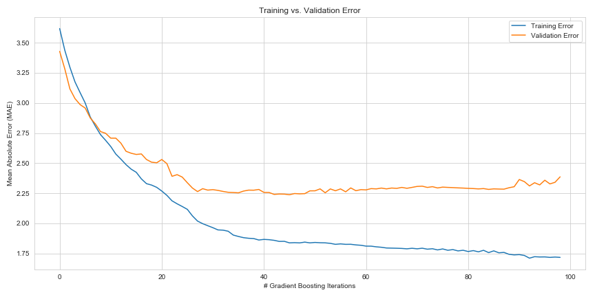
Overfitting can be a problem with any boosting algorithm, and gradient boosting is no exception. Because each new weak learner is focusing on errors that previous learners have made, running gradient boosting for too many iterations typically leads to a highly overfitted model. The best solution is to split your data into three sets, instead of the usual two; train, test, and validation. The validation set error should be separate from the training set (i.e. don’t use your validation set for training), and the error should be evaluated after every boosting iteration. What you can do is stop boosting once your training error begins to converge on your validation error - any further boosting is likely to stop your boosted model’s ability to generalise to new examples.

To show you this, I built a super-rudimentary gradient boosting classifier with the objective of minimising absolute error on the Boston Housing dataset. I held back a portion of the dataset for validation, and plotted training and validation error on each iteration. As you can see, validation error seems to plateau by around the 30th boosting iteration - but training error continues to reduce (albeit, rather slowly) up to the 80th or even 100th iteration (note that over-training actually has a negative impact on validation error, too).

In closing

Gradient boosting takes the concept of fitting on residuals as a form of gradient descent, and generalises it to that of gradients and pseudo-residuals. This generality allows machine learning practitioners to build startlingly accurate classification and regression algorithms with objective functions designed specifically for the application at hand.

Lots of outliers? No problem, just choose absolute error or Huber loss! Building a binary classifier? No problem, just use the zero-one loss. A probabilistic classifier? Use log-loss or hinge loss! This is what makes gradient boosting so flexible, and so powerful - and why it has earned its place in many practitioners’ hearts as the “sensible default”.