Blog

Stochastic Gradient Descent (let’s call it SGD from now on, because that feels a bit less repetitive) is an online optimisation algorithm that’s one of the “core” algorithms in a data scientist’s toolbox. The most attractive things about it are its simplicity scalability - because of how it differs from other gradient descent algorithms, SGD lends itself neatly to massively parallel architectures and streaming data.

A recap of Gradient Descent

Let’s start with a recap of the classic: gradient descent (GD). GD is an iterative optimisation algorithm that takes small steps towards a minimum of some function (notice that I say a minimum instead of the minimum - GD can get caught in local minima if the function is nonconvex and the starting point is poorly chosen). It works by evaluating the output of the objective function at a particular set of parameter values and then taking partial derivatives of the output with respect to each of the parameters. Using these partial derivatives, it’s possible to determine which parameters can be changed to minimise the value of the objective function. Basically, GD looks for the direction that most minimises the objective and then takes a small step in that direction - rinse and repeat until convergence.

An objective function

Let’s jump into some of the maths. The GD algorithm’s objective is to minimise some function $J$ by determining the optimal values of some parameter set $\theta$. This is done iteratively, so a single iteration (a single update of the parameters $\theta$) would look something like this;

$$ \theta = \theta_{old} - \alpha \nabla_{\theta} E\left[ J(\theta; X, y) \right] $$

The interesting thing to note here is that GD requires computing the expected value of the function $J(\theta; X, y)$ over the whole dataset (i.e. $E\left[ J(\theta; X, y) \right]$). That is, the objective function is evaluated over the entire dataset and then averaged - and this happens during each iteration of the GD algorithm. This is fine for smaller optimisation tasks, but this can run into significant problems at scale - evaluating a function over a whole dataset can prove intractable if your dataset is large, or arrives in small pieces (e.g. during streaming).

Gradient descent for linear regression

More concretely, let’s look at the objective for linear regression - mean squared error. In this case, our learning problem has $n$ examples and $m$ features. Let’s define some things up front, so that our objective function makes sense.

• Let $\underset{n \times m}{X}$ be our design matrix - with rows for each training example and columns for each feature (and an additional column for the bias term)
• Let $\underset{n \times 1}{y}$ be a vector holding our target variable - we want to predict $y$ given the data in our matrix $X$.
• Let $\underset{m \times 1}{\theta}$ be our parameter vector - an $m$-length vector containing the coefficients for each feature and the bias term.

In this case, the mean squared error over a dataset $X$ is defined as follows;

$$ J(\theta; X, y) = \frac{1}{2n} (y - X\theta)^{T}(y - X\theta) $$

Note that sometimes practitioners divide this function by a factor of two (i.e. the $\frac{1}{2n}$ at the beginning) so that the derivative is a little bit neater. This isn’t strictly necessary and doesn’t change the overall shape of the function - it’s just a mathematical convenience.

To use gradient descent to optimise $J(\theta; X, y)$, we’d want to begin by setting $\theta$ to some arbitrary values. We then evaluate the function’s gradient at that point to get an idea of the slope of the local area. We then focus on taking a number of small steps “downhill” to update $\theta$ by nudging the weights in the direction that minimises the objective. By taking enough steps this way, we will eventually arrive at an optimum.

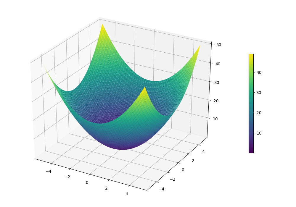
One thing to note here is that the linear regression objective function is quadratic (like the one pictured below). It is therefore convex and has a single global optimum — this isn’t always the case with more complex functions.

Going downhill

Let’s compute the derivative for this objective function - once we’ve done that, we can start stepping down the hill. This involves a little bit of matrix calculus, so I’ve left some extra steps in so that it’s clear what’s happening. Both Cosma Shalizi’s lecture notes and the Matrix Cookbook¹ are really handy here.

$$\begin{aligned} \frac{\partial}{\partial \theta} J(\theta; X, y) & = \frac{\partial}{\partial \theta} \frac{1}{2n} (y - X\theta)(y - X\theta) \\ & = \frac{1}{2n} \frac{\partial}{\partial \theta} \big( y^{T}y - 2\theta^{T}X^{T}y + \theta^{T}X^{T}X\theta \big) \\ & = \frac{1}{2n} \big(-2X^{T}y + \frac{\partial}{\partial \theta} \theta^{T}X^{T}X\theta) \big) \\ & = \frac{1}{2n} \big(-2X^{T}y + 2X^{T}X\theta \big) \\ & = \frac{1}{n} \big(-X^{T}y + X^{T}X\theta \big) \\ & = \frac{1}{n} \big(X^{T}X\theta - X^{T}y \big) \end{aligned}$$

Putting it all together

Now that the derivative of this function is known, we can plop it directly into the gradient descent algorithm. The objective function that we determined earlier computes the expected value over the entire dataset, so we can simply drop it in place. A single round of parameter updates would look like this:

$$ \theta = \theta - \alpha \big( \frac{1}{n} X^{T}X\theta - X^{T}y \big) $$

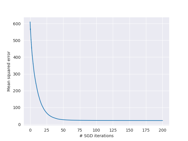
I applied this parameter update to the Boston housing dataset² and then ran GD for 200 iterations with $\alpha = 0.05$. Below is a plot showing the overall error on each iteration - you can see the error begin to converge to a stable state after about 25 iterations;

Now that we know GD works on our linear regression problem, let’s head back over to SGD-land and start tinkering with that instead.

Back to SGD

Right. Now that we’ve recapped standard gradient descent, let’s dive right into the interesting stuff. The update procedure for SGD is almost exactly the same as for standard GD, except we don’t take the expected value of the objective function over the entire dataset, we simply compute it for a single row³. That is, we just slice out a single row of our training data and use that in a single iteration.

$$ \theta = \theta_{old} - \alpha \nabla_{\theta} J(\theta; X_{(i)}, y_{(i)}) $$

Because we’re only computing the gradient based on a single example at a time, we’re going to need far more iterations to converge upon a sensible result. Below, I ran a plot of error convergence after about 10,000 iterations (roughly equivalent to 200 epochs as the full dataset was seen 200 times).

However - as you may expect, updating the parameter vector based on a single training example is going to play havoc with the initial variance in the training error (and the gradient of the parameter vector). This can cause problems initially - because the variance is so high, SGD requires a considerably smaller initial learning rate than vanilla GD.

During the initial few iterations, both the parameter vector and the MSE will initially have far greater variance as the parameters are being updated directly with each training example. As the number of training examples analysed grows larger, the influence of each individual example diminishes and the parameters will start to converge to a steady state.

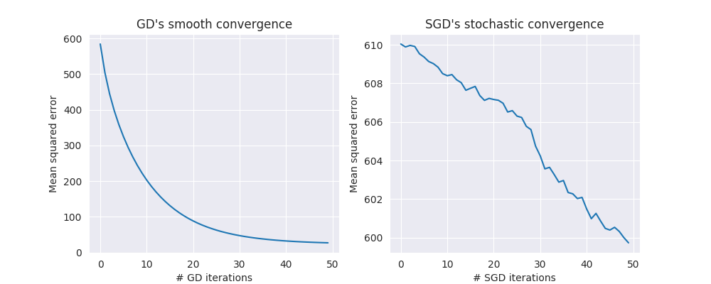
To demonstrate the high variance in SGD, here’s a comparison of the error rate convergence during the first 50 iterations of standard GD (left) and SGD (right)

• note that each GD iteration analyses the entire dataset, while each SGD iteration only analyses a single example (this is also why standard GD seems to converge much faster in this plot).

Disadvantages and traps for SGD

Slow convergence in ravines and valleys

A downside of SGD is that it can struggle on certain types of topographic features, such as functions in “ravines” - a long shallow path surrounded by steep walls. An unfortunate random sequence of training examples can cause SGD to update the parameters $\theta$ such that the objective essentially “bounces” off the walls of the ravine - oscillating between the steep sections but never arriving at the local minimum in the middle.

Typically this is addressed by modifying the algorithm to take into account “momentum”. That is, once the parameters start to converge in a particular direction, a certain amount of “force” is required to overcome that momentum. This helps overcome some of the effects of noisy data by applying a kind of smoothing effect to the parameters, and effectively dampens the oscillations that can occur in ravines and other challenging topographical features.

The implementation of momentum is simple enough. We keep track of a vector $v$ which contains information about the algorithm’s current momentum - and we use a parameter $\gamma \in [0, 1)$ which controls the exponential weighting of past values in the momentum vector $v$. Then, instead of directly updating the parameters with the gradient vector, we update $\theta$ by subtracting our momentum-augmented vector $v$ instead.

$$ \begin{aligned} v &= \gamma v + \alpha \nabla_{\theta}J(\theta; X_{(i)}, y_{(i)}) \\ \theta &= \theta - v \end{aligned} $$

Choosing the correct learning rate

The sensitivity of SGD to individual training examples also means that it’s much more important to choosing a sensible learning rate, $\alpha$. Setting $\alpha$ too high means the algorithm won’t converge smoothly (or that it might oscillate between several sub-optimal states), and setting it too low means that it’ll take far longer to converge than necessary (if ever).

There are several heuristic approaches for determining $\alpha$ that seem to be relatively common in practice. One such example is Leon Bottou’s heuristic⁴ (used in the SGD implementation in sklearn), while several other learning schedules are mentioned in the Stanford Deep Learning materials (this includes approaches like reducing the learning rate as the algorithm begins to converge, or using an optimisation technique like simulated annealing to periodically choose a better learning rate).

Scaling

Something that caught me out when working on my own implementation of this algorithm was poorly scaled input. It turns out that one of the most important things to do before using SGD is to scale your input data to sensible values. Scaling to zero mean and unit variance (typically referred to as “standardisation” in the machine learning literature) is as straightforward as $X_{scaled} = \frac{(X - \bar{X})}{\sigma_X^{2}}$.

Using gradient descent algorithms with unscaled data can cause highly suboptimal results - in the best case scenario, it’ll just cause slow convergence; in the worst case, the gradient will become unmanageable due to numerical precision errors (i.e. the “exploding gradient” or “vanishing gradient”) - which stops the algorithm converging at all.

Dataset ordering

Finally, the ordering of the dataset can bias the way that the gradients develop as SGD is exposed to more of the training data. If there’s some meaningful ordering to the data (e.g. think of horse racing results where race winners are listed in the first row for each race). If this happens over an appreciable number of training examples, then this can cause the algorithm to choose vastly sub-optimal parameter values. There are several ways around this, but the easiest solution is simply to shuffle the dataset before using SGD.

The solution? Mini-batch gradient descent

Mini-batch gradient descent (MBGD)uses, surprisingly enough, small bundles of training examples to optimise the parameters in batches. This is actually quite a neat formulation, as it addresses some of the problems of both vanilla GD and SGD outlined above. Firstly, performing optimisation in small batches of training examples allows programmers to use a vectorised implementation of gradient descent - which is considerably faster than the iterative approach in SGD. However, MBGD is still easy to parallelise as it will typically use a relatively small batch size (e.g. it’s perfectly feasible to use a batch size of 100 to 200 examples).

Secondly, because training happens in batches (even if they’re only small ones) this has the handy side-effect of substantially reducing the variance between iterative applications of the algorithm. Note that this won’t remove all of the variance between iterations - but it will certainly help. Again, a single parameter update with MBGD would look something like this;

$$ \theta = \theta_{old} - \alpha \frac{1}{b} \nabla_{\theta} J(\theta; X_{[i, i + b]}, y_{[i, i + b]}) $$

Note that the batch size here is denoted by $b$ - and the indices on $X$ and $y$ simply indicate a slice of the dataset (i.e. a mini-batch).

In summary

So, that’s SGD in a nutshell. We looked at gradient descent from first principles, and applied it to a standard least-squares linear regression problem setting. We then implemented stochastic gradient descent for comparison, and achieved similar results with some small trade-offs. We looked at some caveats and traps that you should keep in mind when implementing SGD, and finally we proposed mini-batch as a potential best-of-both-worlds compromise between vanilla GD and SGD.

References and further reading