Monopoly is an interesting game. It’s one of the “default” board games that gets wheeled out at every family Christmas, and gets half-heartedly played for a couple of hours - until the players get angry and storms off, anyway. The reason it’s so frustrating is that it’s pretty clear who will win after about half an hour of gameplay - the remaining playtime is just a slow, painful game of attrition during which other players are forced into progressively more desperate financial situations until they lose.

In the interests of keeping future family disputes down to a minimum, I decided to see if there were any mathematical or numerical techniques that I could use to optimise my own playing strategy - thus ending the game as quickly as possible… with as few objects being thrown across the room as possible.

The game that inspired Monopoly was originally designed by an anti-monopolist campaigner who designed the game as a way of educating players about the exploitative nature of unregulated capitalist economies. This is why it’s so frustrating to play - it is specifically designed to show that luck and an unequal distribution of wealth will (in the long run) eventually boil down to a complete monopoly on money and resources.

Dice statistics

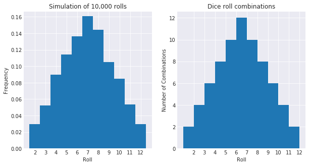
One of the first important things to know is how rolls are distributed when using two dice. Assuming that the dice are fair, there is a uniform probability distribution - that is, it is equally likely to roll any number between 1 and 6. However, rolling two dice and adding the sums together results in a non-uniform probability distribution (thanks to the Central Limit Theorem).

Simulating ten thousand rolls of two dice with uniform probability distributions gives us a pyramid shape - and immediately, it’s clear that the most likely dice roll is 7. This is really a combinatorial problem; rolling a 3 is more likely than rolling a 2 because there is only one way to roll a 2 (i.e. (1, 1)), whereas there are two ways to roll a 3 (i.e. (2, 1) and (1, 2)). Both of these things have been plotted below.

# create ten thousand dice rolls
d1 = np.random.randint(low=1, high=7, size=10000)
d2 = np.random.randint(low=1, high=7, size=10000)

# plot a histogram
rolls = np.arange(2, 13)
plt.hist(d1 + d2, bins=np.arange(1, 13) + 0.5, normed=True)

# show the same thing using combinatorics
dice = [1, 2, 3, 4, 5, 6]
throws = list(itertools.product(dice, dice))
combos = [sum([len(throw) for throw in throws if sum(throw) == i]) for i in rolls]
plt.bar(left=rolls-0.5, height=combos, width=1)

What’s the mean value for a dice roll?

This is an easy one. We can see from above that the value with the highest probability overall is $7$ - but this is the mode, not the mean. We can compute the mean by dividing the sum of the entire state space by the number of states. Interestingly, this also yields $7$ as the average roll (and therefore the most likely). We will use this trick later.

sum(map(sum, throws)) / len(throws)

>>> 7.0

Board Statistics

The Hard Way

This bit is going to need a little bit of legwork. I’m going to build a model of how the players in Monopoly, using the information about probability from earlier. This also includes building a model of game actions that can change a player’s position - for example, landing on a Chance card or going to Jail.

There are several relevant rules for going to/getting out of jail;

• If you draw a certain Chance or Community Chest card, you go to Jail.
• If you roll doubles three times in a row, you go to Jail.
• No prizes for guessing what happens if you land on the ‘Go to Jail’ square…

If you are in jail (which lasts for up to 3 turns), you get to roll the dice each turn. If you roll a double, you get out of jail and progress that number of squares (i.e. 2, 4, 6, 8, 10, 12)

board = np.zeros(n)
jail = 10        # jail is the 11th square (not the 10th - go on, check it)
go_to_jail = 30  # "go to jail" is the 31st square

def roll(d=2):
    return np.random.randint(low=1, high=7, size=d)

def update_position(pos, max_pos=40):
    if pos >= max_pos:
        pos = pos % max_pos

    board[pos] += 1
    return pos

def sit_in_jail(pos):
    pos = update_position(jail)

    # if in jail, roll 3 times (until doubles)
    for i in range(3):
        r1, r2 = roll(2)
        if r1 == r2:  # doubles, out of jail
            pos = update_position(pos+r1+r2)
            assert pos != jail
            break

    # if not rolled a double, roll as normal
    if pos == jail:
        r1, r2 = roll(2)
        pos = update_position(pos+r1+r2)

    return pos

def take_turn(position):
    num_doubles = 0
    while True:
        r1, r2 = roll(2)
        position = update_position(position+r1+r2)

        if position == go_to_jail or num_doubles == 3:
            position = sit_in_jail(position)
            num_doubles = 0

        if (r1 == r2):
            num_doubles += 1
        else:
            break

    return position

pos = 0  # start from "Go"
for g in range(0, 1000):  # simulate 1000 games
    pos = 0
    for i in range(0, 1000): # simulate 1000 turns in each game
        pos = take_turn(pos)

Now that our simulation has been built, let’s visualise what we have…

The Easy Way™

I initially wrote this post a couple of years ago when I was playing with Monte-Carlo-type simulation modelling. During my Master’s degree though, I found out about the magic of Markov chains and how a little bit of linear algebra would make this whole task a lot simpler. Essentially, it’s possible to compute a state transition matrix (i.e. the matrix linking the previous turn to the next) using a little bit of basic matrix multiplication. What’s even better is that the state transition matrices have some neat properties that we can take advantage of. With that in mind, let’s get cracking.

After a little bit of Googling, I discovered that this problem has actually been tackled quite a few times before in various other blog posts. I’ll be drawing on some of the interesting bits from those and working them into this.

One really imprtant thing to note here is that there are two main steps in a Monopoly turn; a first step when the dice are rolled, and the second when any additional movements are carried out (e.g. Go to Jail, Move to Go, etc).

Let’s start with making the dice-roll transition matrix. This takes the form of a Markov stochastic matrix - in short, a square matrix with an entry in each row and column for each square on the Monopoly board. Each row describes a state that the board could be in. Each row in this matrix represents transition probabilities from that state (because this represents a discrete probability distribution, each row will sum to 1).

d = [1, 2, 3, 4, 5, 6]
rolls = np.asarray(list(itertools.product(d, d))).sum(axis=1)
values, counts = np.unique(rolls, return_counts=True)
probs = np.asarray(counts, dtype="float64") / counts.sum()

r_tr = np.zeros((n, n))
for i in range(0, n):
    indices = (i + values) % n
    r_tr[i, indices] = probs

Next, we have to compute the probabilities for the second step in each turn. This includes the community chest cards, chance cards, “Go to Jail” square, and so on.

Note that we don’t have to do it like this - one neat property of Markov transition matrices is that you can “chain” them together with a single matrix multiplication (hence Markov chain, geddit?). Each extra part of a turn (e.g. rolling dice, chance cards, community chest cards, going to jail, etc) can be formulated as individual transition matrices (and then combined later on with a multiplication). However I’m lazy, so I put all of those secondary transition probabilities into a single matrix for simplicity.

jail = 10
go_to_jail = 30

s_tr = np.zeros((n, n))

# rolling doubles 3 times
p_triple = (1.0 / 6.0) ** 3
s_tr[[i for i in range(0, n) if i not in [jail, go_to_jail]], jail] = p_triple

# chance cards
## "go back three squares"
for pos in pos_chance:
    s_tr[pos, (pos - 3)] = 1.0 / 16.0

## go, jail, pall mall, marylebone, trafalgar square, mayfair
chance = np.asarray([0, 10, 11, 15, 24, 39])
s_tr[np.ix_(pos_chance[0], chance)] = 1.0 / 16.0

# community chest cards
## go, old kent road, jail
chest = np.asarray([0, 1, 10])
s_tr[np.ix_(pos_community_chest[0], chest)] = 1.0 / 15.0

# go to jail square
s_tr[go_to_jail, jail] = 1.0
s_tr[go_to_jail, go_to_jail] = 0.0

# rolling doubles while in jail
sq_jail = np.asarray(np.linspace(2, 12, 6) + jail, dtype="int")
s_tr[np.ix_([jail], sq_jail)] = 1.0 / 36.0

# filling in the blanks...
for i in range(0, n):
    s_tr[i, i] = 1 - s_tr[i].sum()

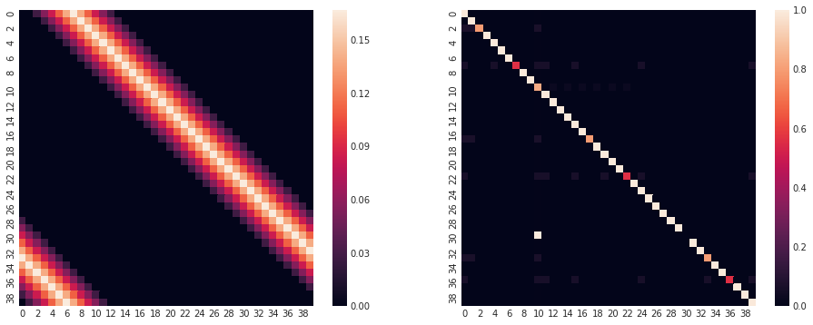
Now that the state transition matrices have been computed, all that’s required to combine them is a single matrix multiplication. Notice the heatmaps below - they represent probabilities of landing on a particular square. In this case, each row ($y$ axis) represents the square that the player is currently on, while each column entry ($x$ axis) represents the transition probability from that point.

For example, let’s look at the left matrix. From the row corresponding to “Go” (row $0$), it appears that the most likely square to transition to (the brightest entry in the row) is square $7$ - or the Angel, Islington. The right-hand matrix shows the transition probabilities for any special cases - Chance cards, Community Chest, Go To Jail, and so on. Notice that the entries in this matrix show much less variation; specifically, this matrix is a lot more similar to the identity matrix - that is, most entries on the diagonal have values close to $1$.

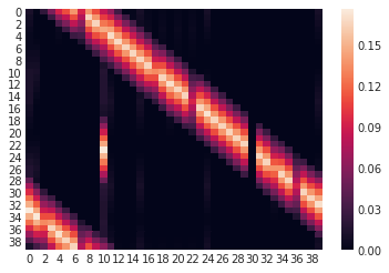
And the final transition matrix from multiplying the two other matrices together…

# compute overall transition probabilities with a multiplication
p = r_tr.dot(s_tr)

Eigendecomposition

OK, so we’ve now got the transition probability matrix for each turn. Now what?

There are two things we can do from here; we can simulate a game by providing a starting state as a vector and then repeatedly multiply this vector with the state transition matrix. With a sufficiently large number of repeated multiplications, the state vector will eventually converge to a limiting distribution - that is, it will reach a state at which further multiplications don’t affect it very much. This procedure is a simple eigenvector approximation algorithm that’s known as power iteration. It will eventually approximate the limiting distribution of the board’s occupation probabilities - that is, the eventual probabilities that each square will be occupied. The power iteration procedure is shown mathematically below;

$$ b_{k+1} = \frac{Ab_k}{|Ab_k|} $$

The other thing we can do is use some of the built-in numerical packages in Python to compute the eigenvalues and eigenvectors for us. The dominant eigenvector (the eigenvector with a corresponding eigenvalue of $1$) that results from this algorithm will show the stationary distribution of occupation probabilities on the board. In theory, this will be faster and more accurate than the power iteration - but in practice the results will be very similar. Let’s go ahead and use the linalg.eig algorithm from the scipy package to compute the dominant eigenvector of this matrix. The goal of eigendecomposition in this case is to find the left eigenvector - a row vector $X_{l}$ satisfying the following equation (where $\lambda = 1$, in the case of a Markov stochastic matrix);

$$ X_{l} A = \lambda X_{l} $$

Note that the eigendecomposition algorithm in the scipy package will compute the eigenvectors corresponding to stationary distributions (that is, state vectors at which repeated transition matrix multiplications won’t change the state). This isn’t always the same as a limiting distribution (which is the result of the power iteration procedure above) - stationary distributions are dependent on the initial input vector, whilst limiting distributions are not. However, we can pick the eigenvector corresponding to the limiting distribution by finding the one with an eigenvalue of $\approx 1$.

u, V = sp.linalg.eig(p, left=True, right=False)
stationary = np.real(V[:, u.argmax()])  # select vector w/ largest eigenvalue
stationary /= stationary.sum()  # normalise so that \sum_{e} = 1
df["mkv_prob"] = stationary

Why the difference between models?

Although slight, there is a clear difference between the probabilities generated by the simulation and the Markov model. Why is this? After a lot of swearing and confusion, I realised something - it turns out that the Markov model’s probabilities represent something ever-so-slightly different to those of the simulation. I wrote the simulation model to record the probabilities of landing on a given square, while the Markov model represents the probabilities of occupying a square at the end of a turn.

This is why, for example, there is such a marked discrepancy between the models for the probability of the “Go To Jail” square - in the Markov model, this square is never occupied as a player landing on “Go To Jail” will immediately move to Jail. However, the simulation model above counts this, as the player will technically land on it but never occupy it.

Property and Property Group Statistics

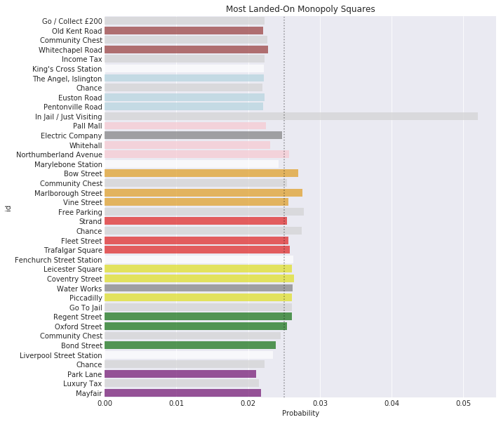
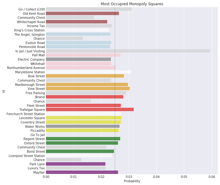
What is the most-occupied property?

It’s fairly well-known that the single most-occupied property is Trafalgar Square, with an occupation probability of just over 3%. Marylebone is a close second - but the most interesting thing is the group of three orange properties (Vine Street, Marlborough Street, and Bow Street) following shortly behind. In this case, the entire orange property group is considerably above average, which suggests that it’s likely to be the most profitable group to own.

One notable thing about the most-occupied squares is that they’re all after the Jail square. When players are sent to Jail (or some other square), they have to resume the game from that point - which has a considerable positive effect on the occupation probabilities of subsequent properties.

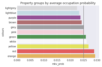
What is the most-occupied property group?

Now that we’ve got an idea which squares are most likely to be occupied, let’s take a look at the average occupation probability per colour group. As I mentioned above, the best property group to own is orange, shortly followed by red, yellow, and white. If you own a set of orange properties, you are about $26%$ more likely to have another player land on them than if you owned a set of light blue properties. Clearly then, it’s all about location, location, location.

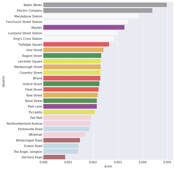
What is the best value property?

This question is a little bit more tricky. Here we have to take into consideration occupation probabilities, as well as the rent/cost ratio of each property. However, this isn’t the whole story - it’s also possible to improve each property with houses and hotels. This complicates our analysis somewhat, so we’ll revisit this later.

There are a couple of things to note here. The Electric Company and Water Works aren’t deterministic in terms of how much rent one is likely to get - so I came up with an average rent based on the average dice roll information that we figured out earlier. Surprisingly, the utilities come out very clearly on top - it seems that they’re the best value initially, shortly followed by the train stations.

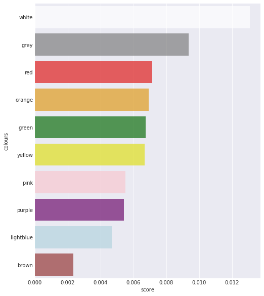
What about property groups?

This is much the same as above, just summed over each particular property group. It appears that the stations are on top, followed by the utilities, and the red, orange, and green properties. Note that the stations come out on top here because there are four of them.

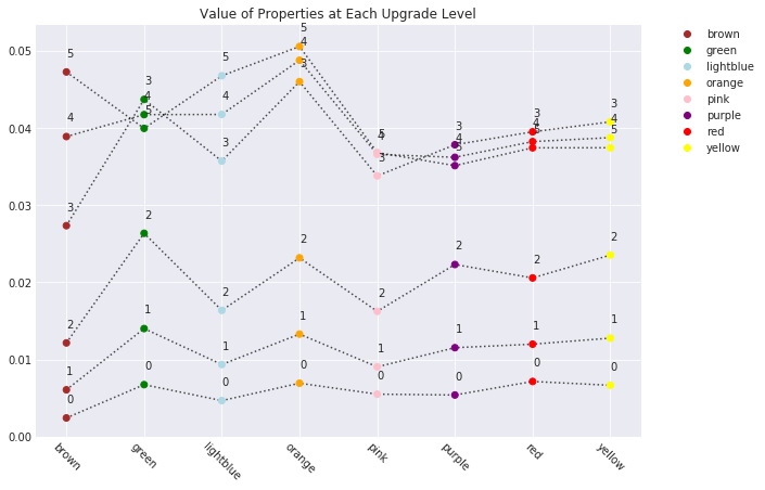
What is the best improvement strategy?

This next question is a little bit more complicated, and the answer is “it depends on the property”. It also depends on how much you can afford to spend on improvements, your strategic goals (for example, using up all of the houses to block other people from using them), and more.

Anyway, there’s a nice chart below to show the results from this part, but I’ll summarise here:

• Generally speaking, overall value is maximised if you build 3 improvements on each property
  • The exceptions to this rule are the light blue and orange groups
• The green properties are excellent value with 3 improvements
• The orange properties are the best overall, with the score for 3/4/5 improvements topping the list
• An honourable mention goes to the brown group - rubbish initially, but much stronger after having 3 or more improvements built

To make a long story short;

• If you’re planning to buy and improve a set of properties throughout the whole game, orange is your overall best bet
• Brown is great value as it offers a good return on investment, is cheap to upgrade, and requires only two properties
• If you’re planning on building on green, build up to 3 houses - but no more

Concluding remarks

Well, this was a really long post. I’ll quickly summarise what we’ve covered and then leave you to (hopefully) never have to think about Monopoly again.

In conclusion;

• Monopoly is a horrible game that will destroy friendships and ruin families
• It’s specifically designed to be as frustrating to play as possible
• The properties with the highest probability of collecting rent are Orange
• The best value properties to invest in are Brown
• Sometimes, it’s not actually worth upgrading properties beyond 3 improvements